

In this project, I play around with different aspects of image warping with a “cool” application -- image mosaicing. I will take photographs and create an image mosaic by registering, projective warping, resampling, and compositing them. We'll be doing this with homographies ;) and use them to warp images.
In part A I play around with diffusion models, implement diffusion sampling loops, and use them for other tasks such as inpainting and creating optical illusions.
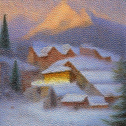
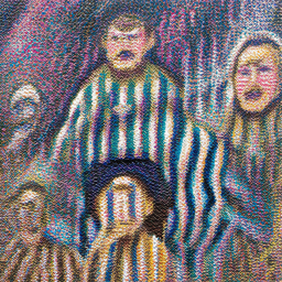
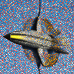
For the 3 text prompts, I display the caption and the output of the model. I also reflect on the quality of the outputs and their relationships to the text prompts.
For num inference steps = 20.


Try a large num_inference_steps=200 (high quality).
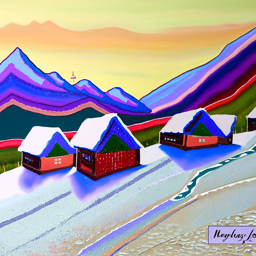
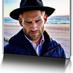
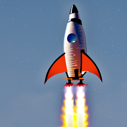
Try a small num_inference_steps=5 (low quality).
A key part of diffusion is the forward process, which takes a clean image and adds noise to it. In this part, we will write a function to implement this. The forward process is defined by: $$ x_t = \sqrt{\bar{\alpha}_t} x_0 + \sqrt{1 - \bar{\alpha}_t} \boldsymbol{\epsilon} \quad \text{where } \boldsymbol{\epsilon} \sim \mathcal{N}(0, 1) $$ Here I take a test image of the Camponile and apply the forward function at levels 0 (no noise), 250, 500, and 750.


Let's try to denoise these images using classical methods. Again, take noisy images for timesteps [250, 500, 750], but use Gaussian blur filtering to try to remove the noise. Getting good results should be quite difficult, if not impossible.


For the 3 noisy images from 1.2 (t = [250, 500, 750]):


In the last part, the denoising UNet does a much better job of projecting the image onto the natural image manifold, but it does get worse as you add more noise. This makes sense, as the problem is much harder with more noise! But diffusion models are designed to denoise iteratively. In this part we will implement iterative denoising . First, I create a list of strided_timesteps. I start at timestep 990, and take step sizes of size 30 until you arrive at 0. My iterative denoise function denoises an image starting at timestep timestep[i_start], applying the above formula to obtain an image at timestep t' = timestep[i_start + 1], and repeats iteratively until we arrive at a clean image. I add noise to the test image to timestep timestep[10] and display this image. Then run the iterative_denoise function on the noisy image, with i_start = 10, to obtain a clean image and display it. I display every 5th image of the denoising loop. I compare this to the "one-step" denoising method from the previous section, and to gaussian blurring.


In step 4, we use the diffusion model to denoise an image. Another thing we can do with the iterative_denoise function is to generate images from scratch. We can do this by setting i_start = 0 and passing in random noise. This effectively denoises pure noise. I will show5 results of "a high quality photo".


The generated images in the prior section are not very good. In order to greatly improve image quality (at the expense of image diversity), we can use a technicque called Classifier-Free Guidance. In CFG, we compute both a conditional and an unconditional noise estimate.


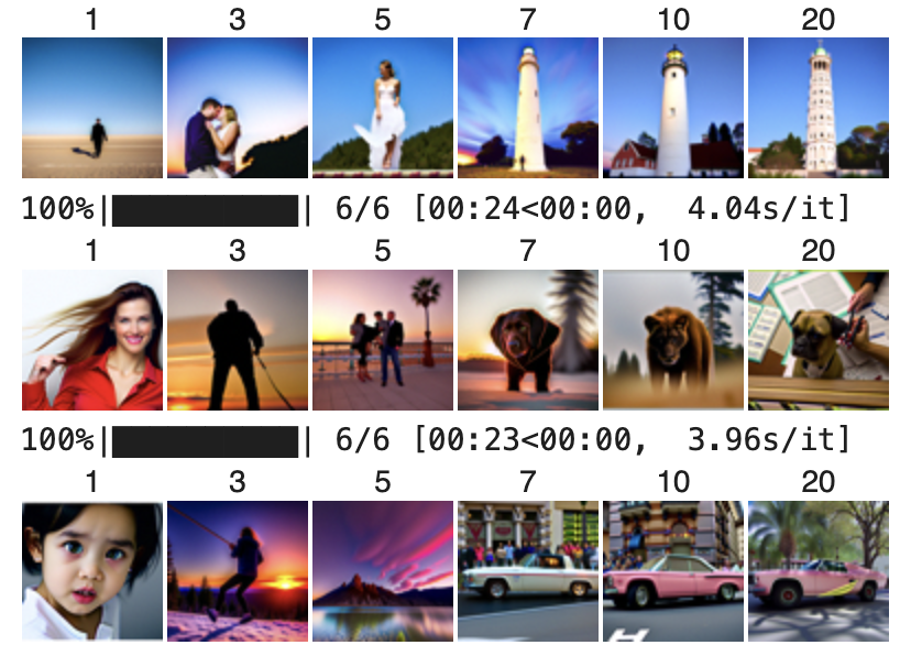
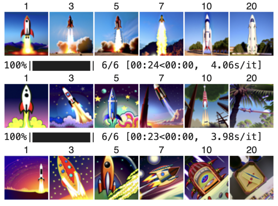
In step 4, we take a real image, add noise to it, and then denoise. This effectively allows us to make edits to existing images. The more noise we add, the larger the edit will be. This works because in order to denoise an image, the diffusion model must to some extent "hallucinate" new things -- the model has to be "creative." Another way to think about it is that the denoising process "forces" a noisy image back onto the manifold of natural images. Here, we're going to take the original test image, noise it a little, and force it back onto the image manifold without any conditioning. Effectively, we're going to get an image that is similar to the test image (with a low-enough noise level). This follows the SDEdit algorithm. Here I show edits of the Camponile image, at noise levels [1, 3, 5, 7, 10, 20] with text prompt "a high quality photo" I do the same with 2 of my own test images.
This procedure works particularly well if we start with a nonrealistic image (e.g. painting, a sketch, some scribbles) and project it onto the natural image manifold. I experiment by starting with hand-drawn or other non-realistic images and see how I can get them onto the natural image manifold in fun ways.


We can use the same procedure to implement inpainting. Given an image and a binary mask, impainting allows us to create a new image that has the same content where is 0, but new content wherever is 1.
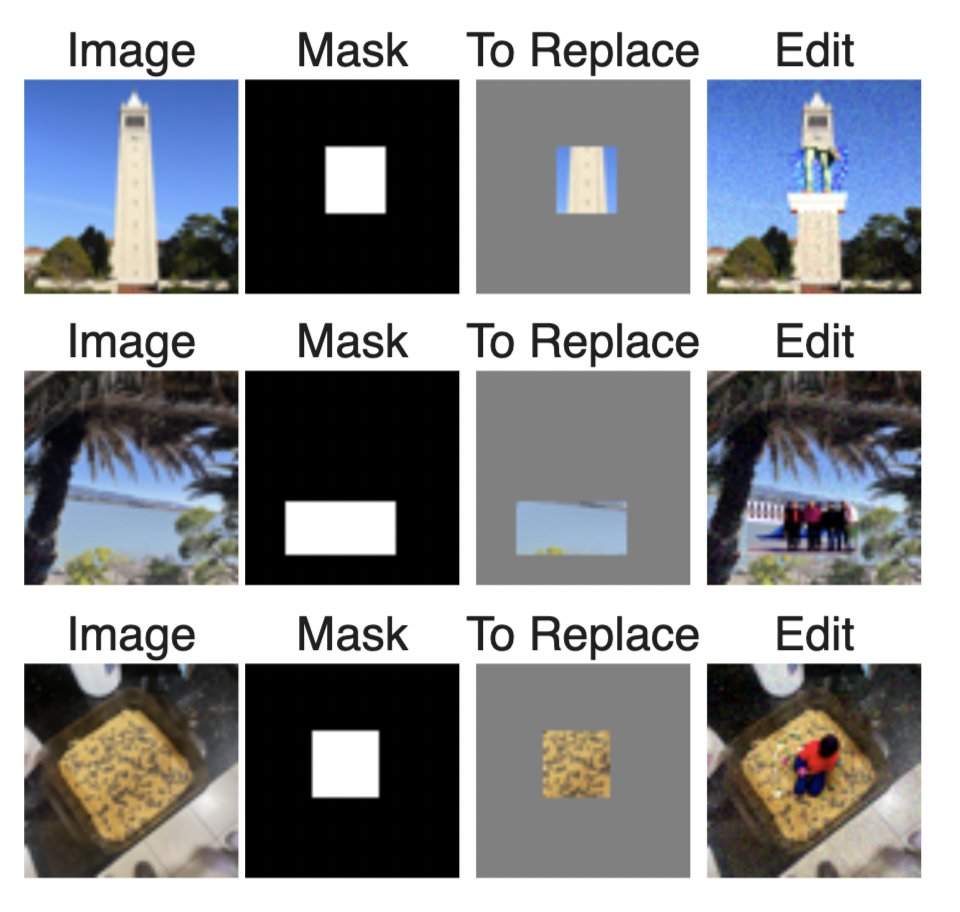
Now we will perform SDEdit but guide the projection with a text prompt.
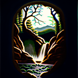
We can also create optical illusions with diffusion models by including an intermediate step in the denoising process. If we want an image that looks like one prompt upside down, but another the right side up, then we can do the denoise step regularly, then flip the image and denoise again, then average the results in each step. We can then perform a reverse/denoising diffusion step with the averaged noise estimate.
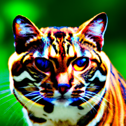
In this part we'll implement Factorized Diffusion and create hybrid images just like in project 2. In order to create hybrid images with a diffusion model we can use a similar technique as above. We will create a composite noise estimate , by estimating the noise with two different text prompts, and then combining low frequencies from one noise estimate with high frequencies of the other.
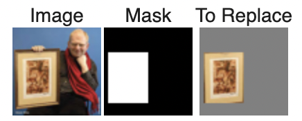
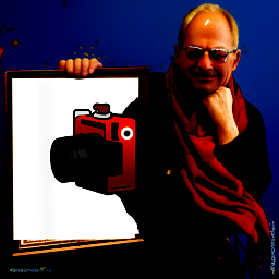
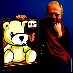
I used SDEdit on a photo of Professor Efros holding up a frame along with a binary mask of the inside of the frame to create two course logos. The first one placed a cartoon camera in it! What was cool about this is it naturally matched the scene so the camera is facing the right way and the colors align!
I will create my own diffusional model from scratch! And train and test it on the MNIST dataset.
Let's warmup by building a simple one-step denoiser. Given a noisy image z, we aim to train a denoiser D such that it maps z to a clean image x. To do so, we can optimize over an L2 loss: $$ L = \mathbb{E}_{z,x} \|D_\theta(z) - x\|^2 $$
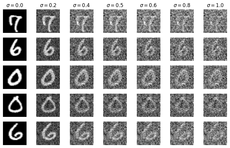
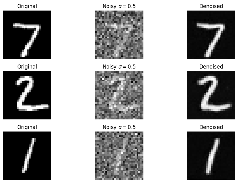
To train our denoiser, we need to generate training data pairs of (z, x) , where each x is a clean MNIST digit. For each training batch, we can generate from using the the following noising process: $$ z = x + \sigma \epsilon, \quad \text{where } \epsilon \sim \mathcal{N}(0, \mathbf{I}). $$ I visualize the different noising processes over different values of sigma.
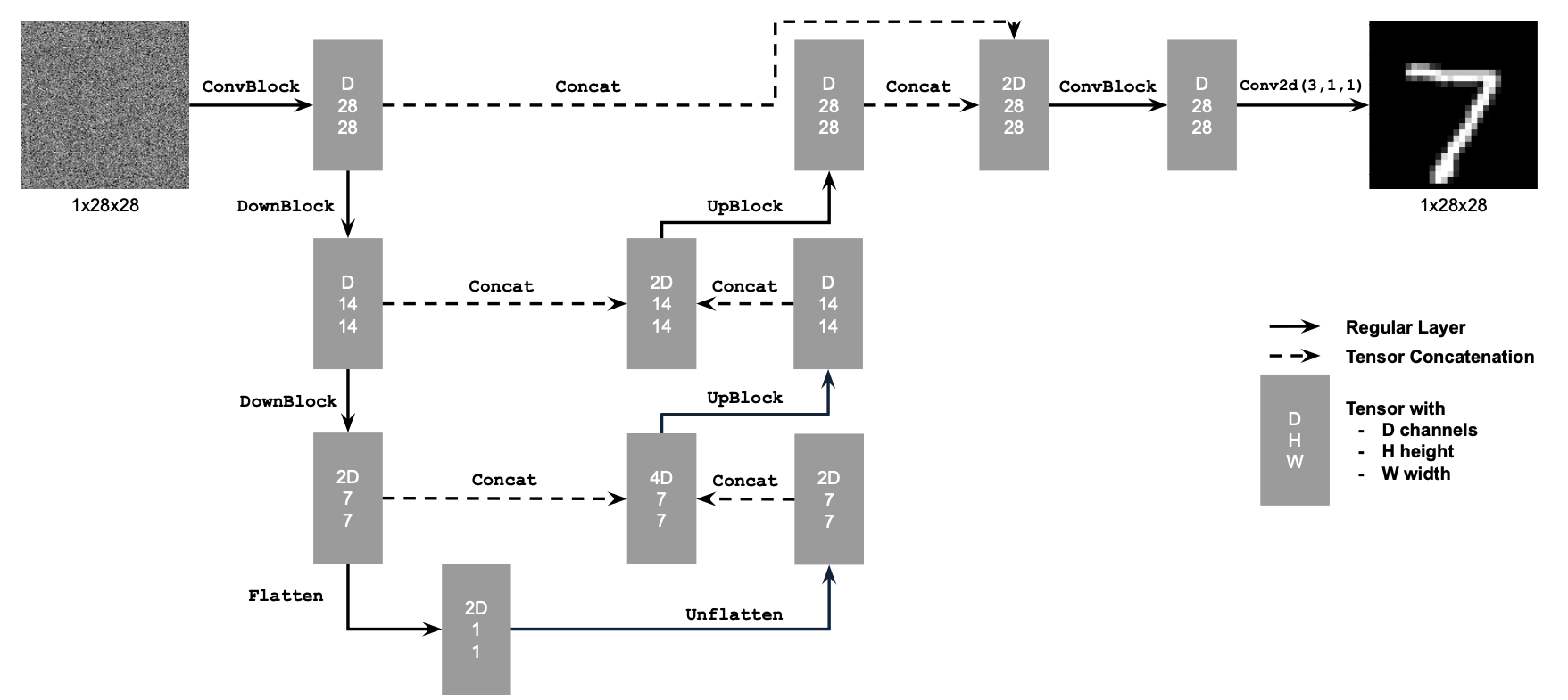
Now, I will train the model to perform denoising. I use the UNet architecture depicted with D = 128 hidden dimension. I use Adam optimizer with learning rate of 1e-4.
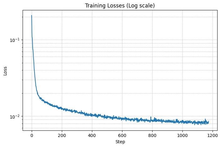
Here I display sample results after the 1st epoch.
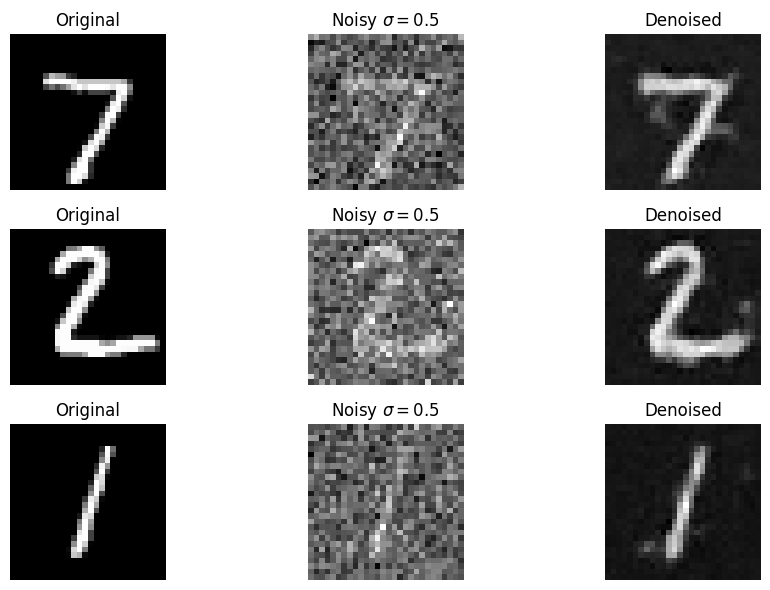
Sample results after the 5th epoch.
I took the original 7 and the denoised 7 and visualized them as a 3D mesh.
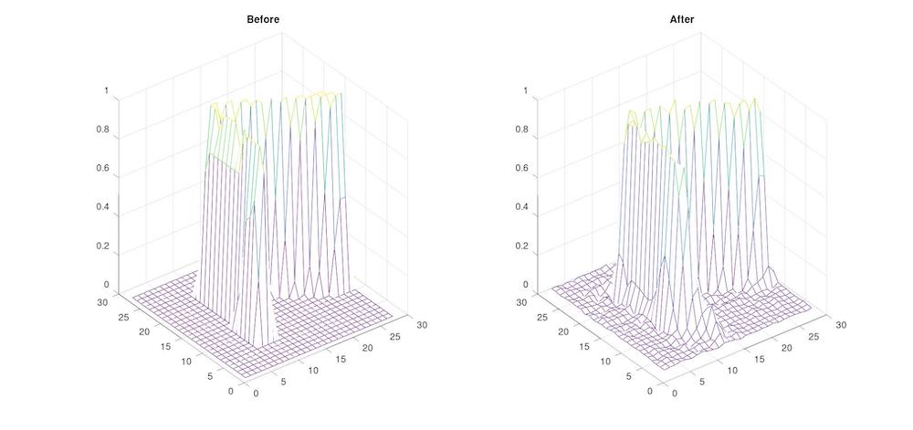
This is interesting because it shows that the noise operation is not compeltely invertable. We see a bit of the added noise around the edges of the 7!
Our denoiser was trained on MNIST digits noised with epsilon = 0.5. Let's see how the denoiser performs on different epsilon values that it wasn't trained for.
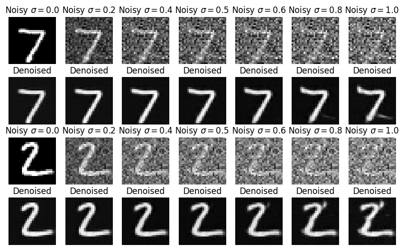
Now, we are ready for diffusion! I will train a UNet model that can iteratively denoise an image. Before, our UNet predicted the clean image. Now, we can change our UNet to predict the added noise (like in part 4A of the project). However, we saw in part A that one-step denoising does not yield good results. Instead, we need to iteratively denoise the image for better results. Our final objective function is: $$ L = \mathbb{E}_{\boldsymbol{\epsilon}, \mathbf{x}_0, t} \left\| \boldsymbol{\epsilon}_\theta(\mathbf{x}_t, t) - \boldsymbol{\epsilon} \right\|^2 $$
We need a way to inject scalar t into our UNet model to condition it.
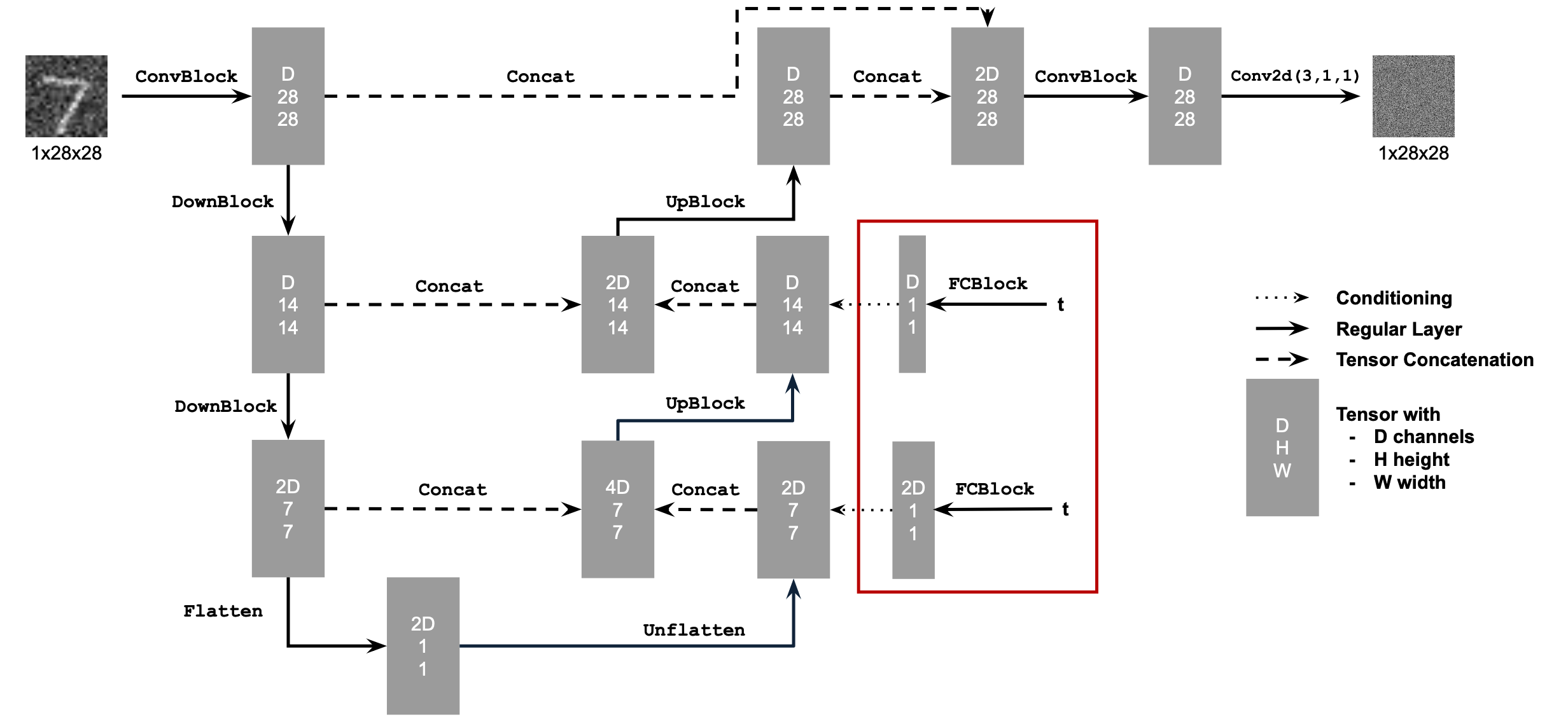
This uses a new operator called FCBlock (fully-connected block) which we use to inject the conditioning signal into the UNet:

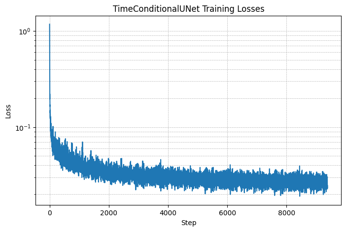
Training time! Basically, we pick a random image from the training set, a random t, and train the denoiser to predict the noise in We repeat this for different images and different values until the model converges and we are happy. I use a batch size of 128 and train over 20 epochs. I again use Adam optimizer, this time with an initial learning rate of 1e-3. I also use an exponential learning rate decay scheduler with a gamma of $$ 0.1^{\left(1.0 / \text{num\_epochs}\right)} $$ This can be implemented using scheduler = torch.optim.lr_scheduler.ExponentialLR().
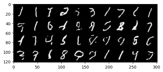
Sampling results for the time-conditioned UNet at 5 epochs.
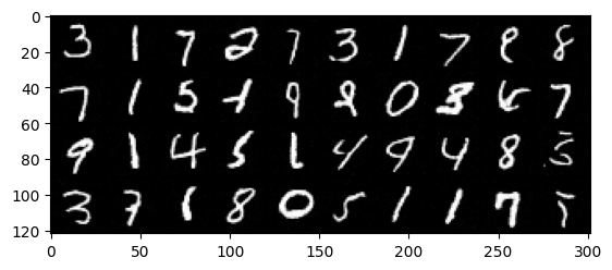
Sampling results at 20 epochs.
To make the results better and give us more control for image generation, we can also optionally condition our UNet on the class of the digit 0-9. This will require adding 2 more FCBlocks to our UNet. Because we still want our UNet to work without it being conditioned on the class, we implement dropout where 10% of the time we drop the class conditioning vector
by setting it to 0.

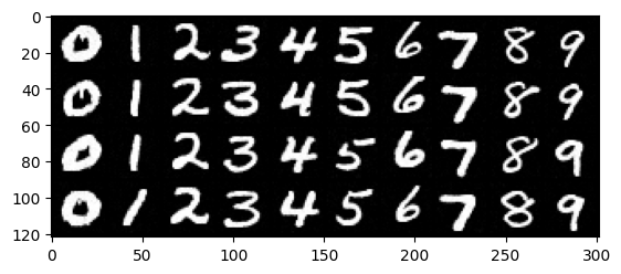
Sampling results for the class-conditioned UNet for 5 epochs. I generate 4 instances of each digit.
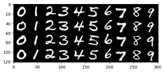
Samplings results at 20 epochs.
It's really cool that diffusional models can seemingly produce images from complete noise!