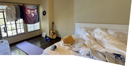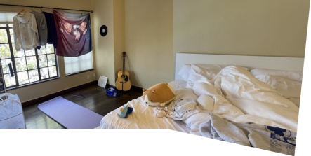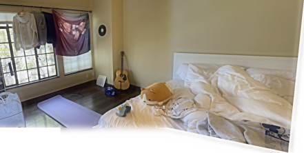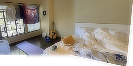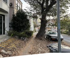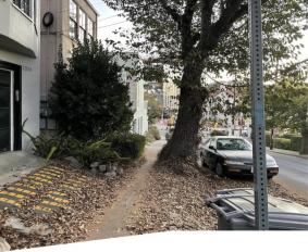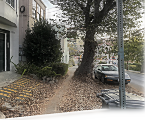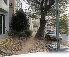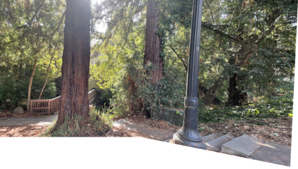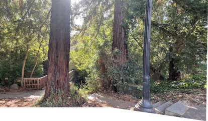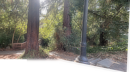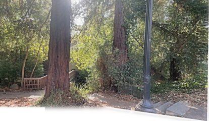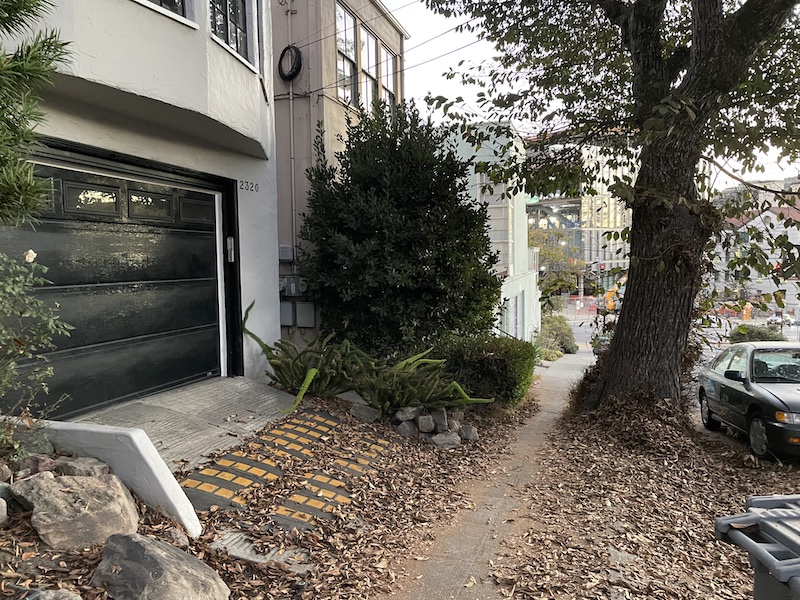
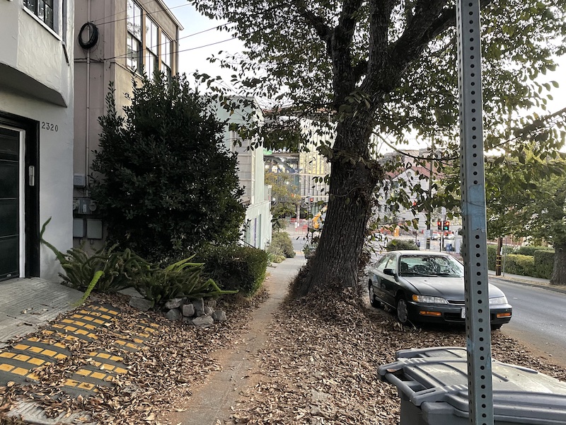
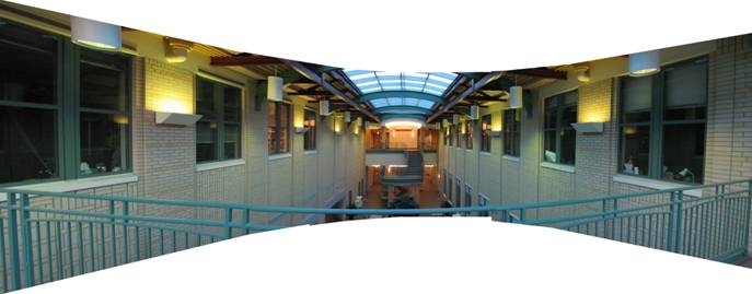
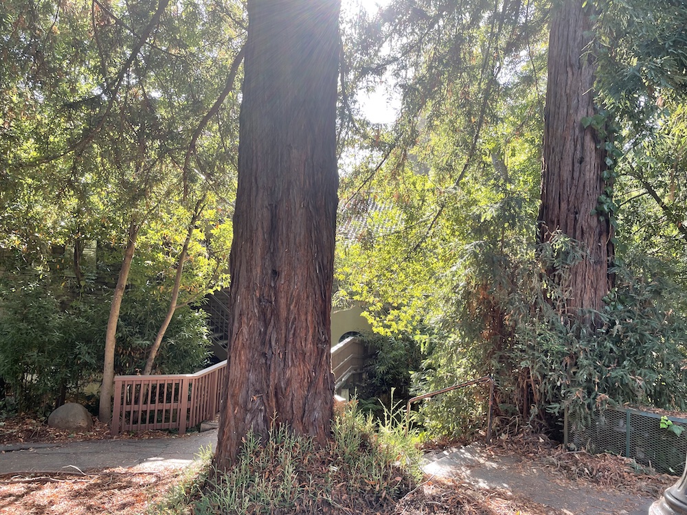
In this project, I play around with different aspects of image warping with a “cool” application -- image mosaicing. I will take photographs and create an image mosaic by registering, projective warping, resampling, and compositing them. We'll be doing this with homographies ;) and use them to warp images.
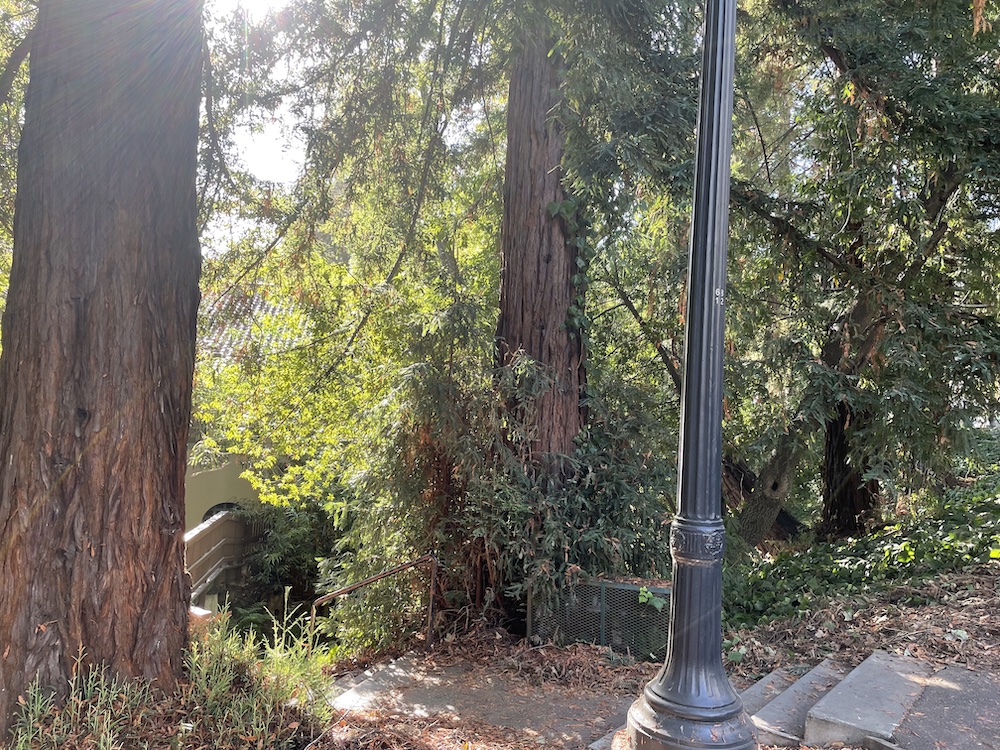
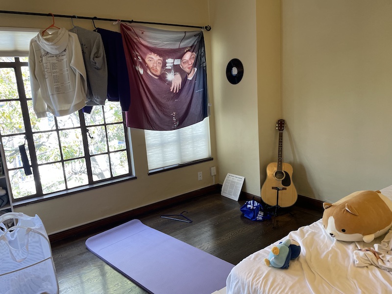
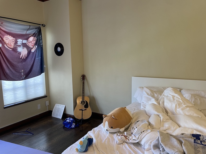
I shot some pairs of pictures at the same center of projection (meaning all I did was rotate the camera around its axis). It's important to maintain the same COP because otherwise we create a new variable, depth, and our homography cannot handle this!


A homography is a projective mapping between any two images with the same center of projection. Given a pair of correspondences betwen the two images, we can recover the homography to warp one image into another. Let's setup a matrix for this, where (x,y) is a correspondence in the source image and (x', y') is a correspondence is the destination image. \[ \begin{bmatrix} a & b & c \\ d & e & f \\ g & h & 1 \end{bmatrix} \begin{bmatrix} x \\ y \\ 1 \end{bmatrix} = \begin{bmatrix} wx' \\ wy' \\ w \end{bmatrix} \]
Expanding into a linear system... \[ \begin{aligned} ax + by + c &= wx' \\ dx + ey + f &= wy' \\ gx + hy + 1 &= w \end{aligned} \] Substituting the last equation. \[ \begin{aligned} ax + by + c &= (gx + hy + 1)x' \\ dx + ey + f &= (gx + hy + 1)y' \end{aligned} \]
Which simplifies to this in matrix form:
\begin{bmatrix} x & y & 1 & 0 & 0 & 0 & -xx' & -yx' \\ 0 & 0 & 0 & x & y & 1 & -xy' & -yy' \end{bmatrix}
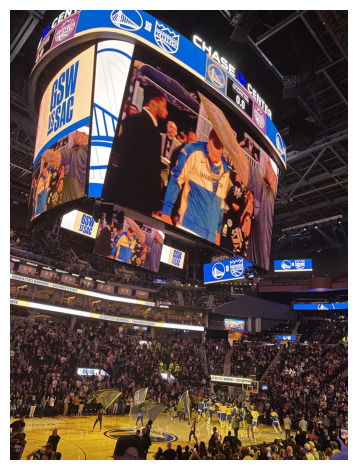
Let's rectify some images! Since the homography requires correspondences on the source and destination image, and for these we don't have a "destination." We can specify points in the desired polygon we want to rectify to. For example, in the Steph Curry screen, I would select the four corners on the source image, and since we know that the screen is a rectangle, we would guess the width and height of a rectangle and use it as the destination correspondences. Same with the fish tank, I know the tank is a square so I use this information for the destination points.
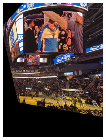
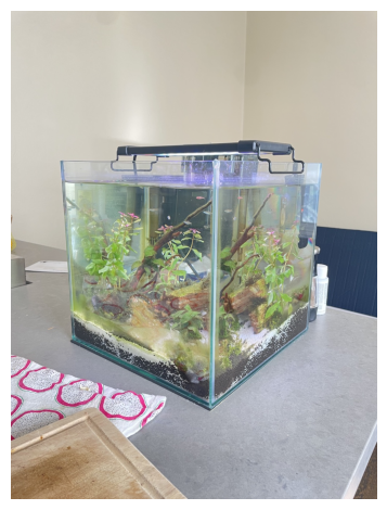
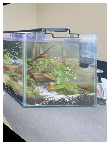
First I naively aligned the images by taking a correspondence point on the image we are warping, then applying the homography to it. We take the difference between this warped correspondence point and the old one, to get how much we should translate the image.


These look pretty good! But notice that on the 1st and 3rd especially you can make out where the two images are stacked since the lighting isn't perfect.
In order to fix this, I implemented a 2-band “Laplacian Stack” blending. I reused some of my code from Project 2 in order to get a Gaussian blur on the full mosaic for the low frequencies and then I computed the Laplacian stack to get the high frequencies of the warped and unwarped seperately (before aligning them into the mosaic) so that only one image's high frequency is operating a time. If we didn't seperate the images, we would get awkward borders on the high frequencies where the two images meet.
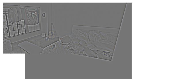
I then added the low frequencies to the high frequencies to produce a smoother transition between images for the final mosaic.

Now the edge looks much smoother! We can repeat this on the other mosaics, too.


Currently I'm manually selecting correspondences for the homography... but what if we wanted to automate this process? In the second half of the project, I will incorporate automatic feature matching and auto-stitching. For steps 1-3, I will implement an algorithm from the paper “Multi-Image Matching using Multi-Scale Oriented Patches” by Brown et al. but with several simplifications.
We want to choose points for our correspondences that are easy to find on both images. The best objects in a scene to do this are "corners," which are formally defined as points in the image with significant changes in all directions. I'll detect this by looking at peaks in the second moment matrix M. $$ M = \sum_{(x,y) \in W} \begin{bmatrix} I_x^2 & I_x I_y \\ I_x I_y & I_y^2 \end{bmatrix} $$ We want to know specifically, in which directions does it have the smallest/greatest change? And since we don't care for any exact values, we just want the general shape of M, we can approximate it by looking at its eigenvalues. For example, case where our image only has derivatives in the x or y direction, our matrix is now axis aligned. We'd just want both eigenvalues to be large and similar in size for that point to be a corner. A good way to write this out is via the corner response function R. $$ R = \frac{\det M}{\operatorname{Trace} M} $$ Now, to detect a corner we just look for points with large values of R, and then threshold accordingly.
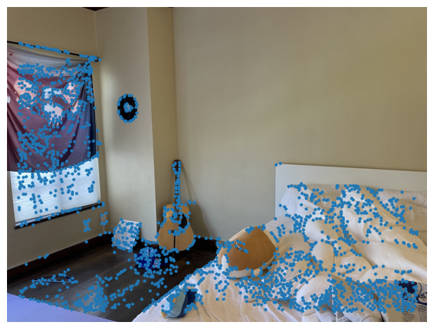
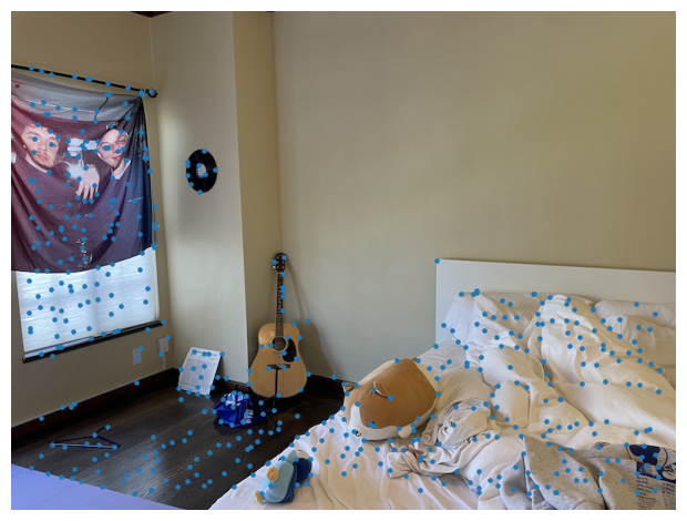
Two issues with the image above is that correspondences and clumped too close together and are not evenly distributed spatially. I implemented ANMS to remedy this. The intuition behind this algorithm is that we are essentially scanning over a radius and only including the correspondence with maximum Harris corner strength within this allowed distance. This radius is dynamically determined per interest point. For each point, we find the minimum radius such that we see another point with a similar corner strength (enforced through C): $$ r_i = \min_j \, |\mathbf{x}_i - \mathbf{x}_j|, \; \text{s.t.} \; f(\mathbf{x}_i) < c_{\text{robust}} f(\mathbf{x}_j), \; \mathbf{x}_j \in \mathcal{I} $$ Now we have a list of minimum radii for each Harris corner in step 1. Finally, we output the first 500 interest points of maximum radius.
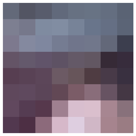
Now that we know how to detect correspondences, how do we match them? I implement Multi-Scale Oriented Patches (MOPS) which takes each point and computes a descriptor vector to best represent the information around that correspondence:
We now have two images, each with their own collection of MOPS descriptor vectors, and are tasked with finding pairs of correspondences. I first implemented a naive nearest neighbor solution: for every patch in image 1, find the most similar patch in image 2 by its L2 distance. The main problem with this solution is that this assumes that every interest point in image 1 has a matching point in image 2. But we know this isn't true since the images contain different views! Thus we need a way to eliminate these "outliers": corners in image 1 but not image 2. I use Lowe's trick for this, which is based off the idea that if the first nearest neighbor isn't that much better than the second, it must mean there isn't a good match. I take the distance 1-NN/2-NN and only include matches with a ratio <= 0.1 (based off of Figure 6 in paper).
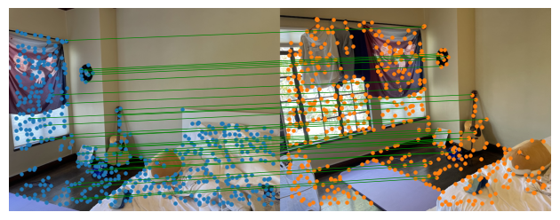
The last problem we need to fix is since we are using least squares to the homography, we REALLY need to make sure there are no outliers. I will use the RANSAC iterative method, which is based off the idea that the general consensus of a group is more accurate than any "expert." The RANSAC loop:
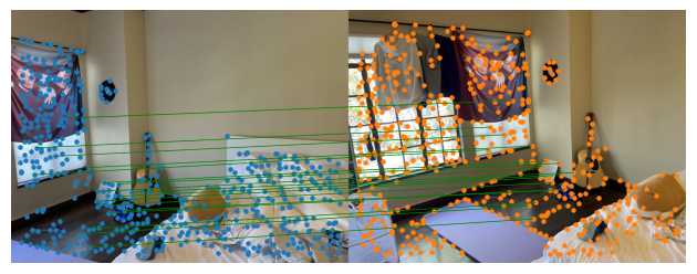
I reran the mosaic pipeline on the three images, but this time using automatic feature detection and matching.
I had a lot of fun implementing this project! Before even starting, it amazed me that images are 2D and have no information about depth, and still our brain pieces together "depth"-like information based off experiences. This means that we can tell in a 2D image what is in front and behind another without seeing the scene in real life. While reading Brown's paper, I found the Harris corner detection method to be really cool. There are so many uses for gradients and calculus turns out to be very simple!
